Research

Sparse regression tries to find the smallest set of input variables that still explains your data well, instead of using all of them. I wrote a solver for a harder version of this problem and benchmarked it against skglm's non-convex solver on synthetic data.

The problem

Sparse regression looks for a weight vector with mostly zero entries that still predicts y from X accurately. The standard convex approach, the Lasso, penalizes the sum of absolute weights. This project instead targets a non-convex fractional penalty, which pushes harder toward exact sparsity but introduces non-convexity. IRLS (Iteratively Reweighted Least Squares) is a standard way to approximate this kind of penalty by solving a sequence of easier weighted least-squares problems, but a plain IRLS scheme for a non-convex penalty can be unstable or converge to a poor solution.

What I implemented

I implemented a modified IRLS solver (irls-f) that adds two things to stabilize the non-convex fit:

Adaptive weights. Each iteration re-weights every coefficient from its current magnitude, driving shrinking coefficients toward zero faster.
A dynamic smoothing term (epsilon). Instead of a fixed small constant, epsilon is recomputed every iteration from the tail of the coefficient magnitudes past the target sparsity level, floored so it never hits zero, and only allowed to shrink.
Each weighted sub-problem is solved with a Cholesky factorization of the weighted normal equations rather than a general linear solve.

The math

The objective being minimized:

\min_{\beta \in \mathbb{R}^p} \; \frac{1}{2} \| y - X\beta \|_2^2 + \lambda \sum_{j=1}^p |\beta_j|^{1/2}

Each IRLS step solves a weighted least-squares problem, where a coefficient the solver currently believes is large is penalized less:

\min_{\beta} \; \frac{1}{2} \| y - X\beta \|_2^2 + \frac{\lambda}{2m} \sum_{j=1}^p \frac{\beta_j^2}{\eta_j}

The weights come from each coefficient's own magnitude:

\eta_j = \left( \beta_j^2 + \epsilon^2 \right)^{\frac{2 - q}{2}}, \qquad q = \tfrac{1}{2}

and the smoothing term $\epsilon$ is recomputed every iteration, floored so it never reaches zero and only ever allowed to shrink:

\epsilon = \max\!\left( \epsilon_{\min},\; \min\!\left( \epsilon_{\text{old}},\; \left( \frac{\sum_{j=k+1}^{p} r(\beta)_j^{\,2-q}}{p} \right)^{\frac{1}{2-q}} \right) \right)

A note on that penalty term: the standard IRLS majorizer for this penalty calls for a $\lambda/4$ coefficient here, but the current implementation uses $\lambda/(2m)$ instead. I'm correcting this (see Results below).

Benchmark

I set this up as a BenchOpt benchmark: the solver runs against a synthetic dataset and logs objective value, reconstruction error and timing every iteration. I compared it against skglm's non-convex solver on the same data and plotted final reconstruction error across both solvers and sample sizes as a boxplot.

Results

Across 80 (sample size, seed) runs logged for each solver, taking each run's final row: skglm reaches the lower objective value in all 80 of 80 runs (median 641 vs. 912 for irls-f), while irls-f has the lower reconstruction error (median 0.0075 vs. 1.03 for skglm). Both are true at once; neither solver wins on both measures.

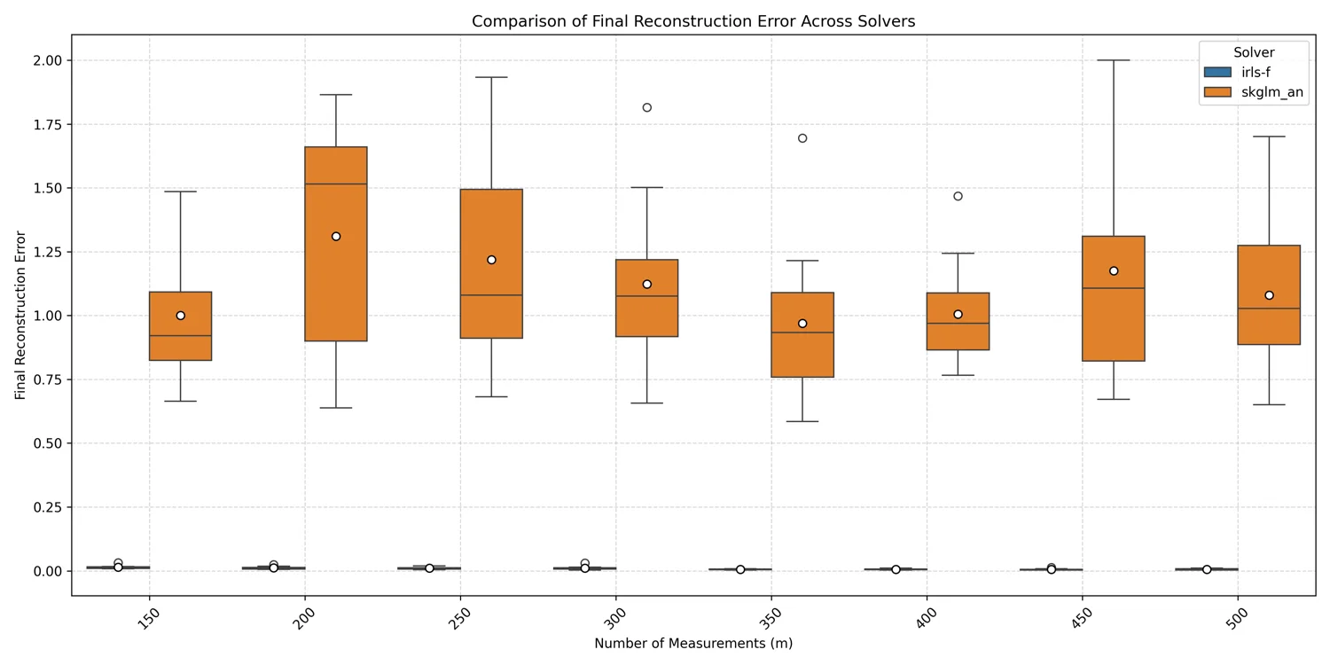
Boxplot comparing final reconstruction error between the irls-f and skglm solvers across sample sizes — Final reconstruction error by solver and sample size, across 80 runs each.

While writing this up I found that my IRLS solver weights the penalty differently from the benchmark objective, so the two runs were not solving exactly the same problem. I'm correcting the scaling and will re-run the comparison.

What's next

I'm currently studying and relearning some textbooks as I continue my IRLS research, and eventually plan to start a new research project in machine learning optimization.